Historical Image Analysis of Tree Mortality at Horseshoe Lake
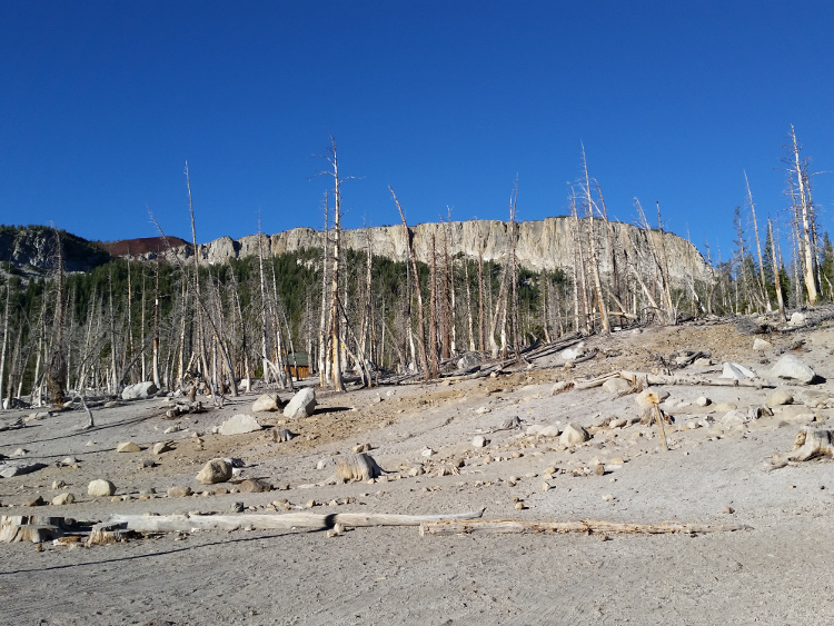
Looking west at the Horseshoe Lake tree kill (July 2016)
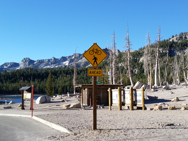
Looking south at Horseshoe Lake tree kill abutting healthy forest (July 2016)
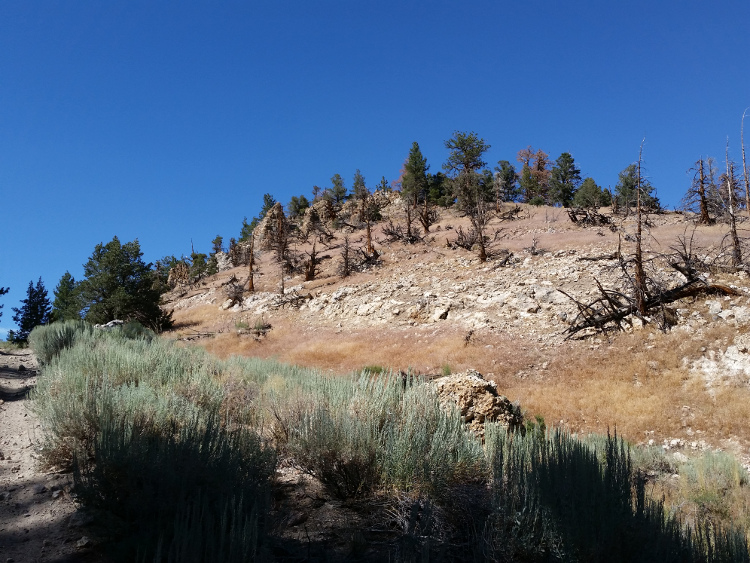
Tree and sage die-off at Basalt Canyon (July 2016)
Read conference abstract View conference poster (PDF)
Duration: June 2016 - October 2017
Affiliation: US Geological Survey
What: Federal research project
My Role: Intern-turned-employee, and occasional field assistant
The Task
I joined the USGS Menlo Park office as a NAGT intern upon my college graduation. The USGS/NAGT Cooperative Field Training Program matches top-performing recent grads with USGS research projects nationwide. I was matched with a photogrammetry and landscape change analysis project within a research group focusing on hydrothermal systems.
This project’s study site was Horseshoe Lake, a recreation area southwest of Mammoth Mountain in Mono County, California. USGS scientists had been studying a unique case of tree dieoff there for a few years, caused by extremely high soil CO2 flux. (More info here.)
My PIs and mentors wished to answer the questions, “How much barren area was present at Horseshoe Lake before magmatic CO2 flux became so high? How has the tree kill area changed over time, and what is the area of this tree kill today?”
Project Goals
- Acquire more photographs for the time series to be analyzed, especially those from pre-1990—to establish a vegetation baseline before regular CO2 monitoring of the site began.
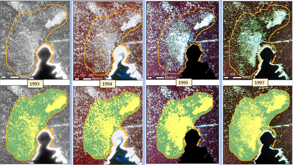
- Develop a consistent image classification method for all the photographs, to quantify the area (m2) of barren ground caused by tree kill.
- Compare the photographs to spatial geochemical data showing the locations of CO2 hotspots over time (Werner et al, 2014) to find spatial patterns or correlations between CO2 spikes and localized pockets of dieoff.
My Approach
I experimented with many image classification methods to select the most suitable method for my historical photographs. This involved reading and synthesizing a lot of seemingly unrelated literature (i.e. machine learning, computer vision) to pick the best technique for my case.
Preliminary tests showed that small differences in the spectral signatures used to “train” the landcover classes led to very large differences in classified image output. To counteract this variation, I took a Monte-Carlo approach: classify each photograph 1000 times based on a random subset of training spectra, and create a final land cover classification based on the average of these 1000 runs.
To control for the effect of image artifacts (i.e heavy shadow) on classification accuracy, I also conducted a landcover classification at an unchanging control site in each photograph, using the same 1000 signature files on which our HSL classifications were based. If the estimated tree-covered area at the control site in a particular image was 25% lower than the mean across the study period, for example, we considered this a 25% under-estimation of the true tree cover due to image artifacts. I could then state whether our HSL classifications under- or over-estimated tree cover and by how much.
Findings
- Between 1951 and 1987, canopy cover at Horseshoe Lake remained relatively constant, with bare ground area beginning to increase in 1992.
- Though field observations seemed to indicate that dieoff had stabilized by 2005, our results show more fluctuation in treeless area than expected after that date—possibly due to significant plant regrowth and large windstorms causing tree fall.
- Despite subsequent spikes in CO2 flux in the region, the footprint/extent of tree kill remained stable from 2001-2014.
Outcome Highlights
- Gained extensive practice in manual georectification of historical images and technical familiarity with various warps used when georectifying
- Sourced historical photographs from EROS EarthExplorer and the Map & Imagery Laboratory at UC Santa Barbara, and added XX new images to the project’s imagery timeline.
- Improved the classification accuracy from previous summer’s work
- Worked very independently with regular status updates to supervisor.
Sources cited on this page:
Cook et al, 2001
Lewicki et al, 2014
Werner et al, 2014