ArcFootprint

An ArcTool for Flux Footprint Estimation

Full Report PDF Download toolbox .zip

Duration: Oct 2019 - Dec 2019
Affiliation: Yale School of Environment
What: Open-source tool
My Role: Sole analyst and report author

The Problem:

I’d seen my colleagues at USGS and Yale calculate gas flux footprints using software that came with their pricey trace gas sensors and flux towers. If you didn’t want to use a proprietary or instrument-specific program, there are open-source methods for gas flux footprint calculation… but many require a standalone software package or advanced programming skills. In addition, if one wants to compare these flux footprints to other spatial datasets in ArcGIS (a standby for many), multi-step conversions are needed to port the footprint results into Arc.

Project Goals:

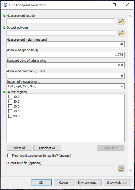
Our term project in Dana Tomlin’s Geospatial Software Design course challenged students to program a custom ArcToolbox tool. I sought to create an easy to use GUI that allows anyone to calculate a 2D flux footprint estimate directly within ArcGIS, where they can input data they’ve collected on their own to just to visualize others’ flux data for mapping purposes.

• Build a user-friendly, point-and-click ArcToolbox tool for generating spatial extents of flux footprints (as shapefiles), based upon meteorological variables collected from gas sensors.
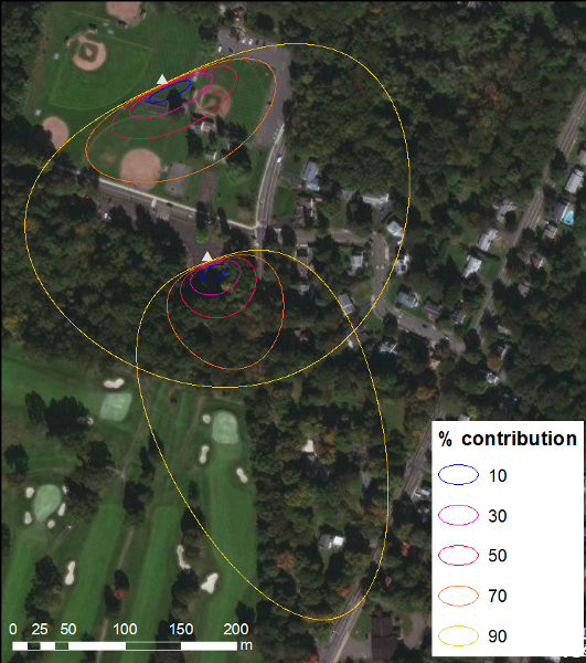
• Construct separate polygons for each source area (50%, 90%, etc.), making it easy for the user to run subsequent Zonal Statistics within each zone.
• Create a tool that will not only benefit my own academic research, but hopefully benefit others conducting meteorological research as well.

Outcome highlights:

The ArcTool consists of two parts: The FFP() function constructed by Kljun et al (2015) for trace gas flux calculation, and a “wrapper” that allows the function’s output ellipses to draw as shapefiles rather than plot in a Python window. Some ArcMap-specific features I’ve added include:

Altering the drawing order of the ellipses, so that the smallest flux source area always appears on top. This order makes symbolizing the flux footprint in maps slightly easier.

arcpy.CalculateField_management(polygons, "footptAREA", "float(!SHAPE.area!)", "PYTHON")
arcpy.Sort_management(polygons, polygonsSorted, [["footptAREA", "DESCENDING"]])

Linear units are automatically converted, if necessary. The output flux footprint ellipses share the same coordinate reference system (CRS) as the input sensor location. If the input point CRS uses meter units, aka if spatial_ref.metersPerUnit == 1.0:, proceed with arithmetic. If not, then:

else:
	# save a factor to convert other-units to meters
	conversion = float(spatial_ref.metersPerUnit) 
	for boundary in xrs: # for each requested footprint outline...
		boundxlist = []
		for vertex in boundary: # for each vertex in a given footprint outline...
			newx = originx + (vertex / conversion) # returns number as Double
			boundxlist.append(newx) # append translated X-value to list
		newxshapes.append(boundxlist)

# repeat for y coordinates

A drop-down menu in the GUI lets the user select the observation season as a proxy for atmospheric boundary layer height (BLH). The height of the boundary layer can change dramatically throughout the year and is a significant parameter in the calculation of flux footprints. I created a simple key:value dictionary that selects a suitable BLH estimate to be used in the flux footprint function, based on observation season.

#look up average values of boundary layer height
seasondictionary = {"Summer (June, July, Aug)": 1000,
		"Fall (Sept, Oct, Nov)": 600,
		"Winter (Dec, Jan, Feb)": 300,
		"Spring (March, April, May)": 1200,
		"Unknown":775} 

#returns the boundary layer height value as a number
PBLH = float(seasondictionary[season])

« Back to Projects